Climate Models
CMIP6
For analysing future climate scenarios, understanding climate variability in a multi-model framework, and assessing climate change impacts, the CMIP6 multi-model ensemble is used. CMIP is a large international effort to advance climate model development and improve scientific understanding of the Earth system, coordinated by the World Climate Research Programme (WCRP) through its Working Group on Coupled Modelling (WGCM)More than 30 research groups worldwide contribute to CMIP6. In total, 21 model intercomparison projects were endorsed for their relevance to the WCRP’s Grand Challenges and the core scientific questions of CMIP6. The model simulations produced within CMIP6 have also been evaluated and used in major international climate assessments and negotiations, including the IPCC Assessment Reports.
The data produced by CMIP6 forms the foundation for the impact models used in the ISIMIP (Inter-Sectoral Impact Model Intercomparison Project), which underpin the results presented in Climate Impacts Online.
Read more about CMIP6: www.wcrp-climate.org
ISIMIP3b
For the Climate Impacts Online web portal, bias-adjusted ISIMIP3b climate input data from the Inter-Sectoral Impact Model Intercomparison Project (ISIMIP) were used. This dataset is based on original global climate model (GCM) outputs from the CMIP6 archive. More information on this dataset can be found on the ISIMIP website
For bias correction and statistical downscaling, the ISIMIP3BASD method and W5E5 v2.0 observational dataset were applied (Lange, 2019a; Lange, 2020).
The data covers three time periods:
- - Pre-industrial (1601–1849)
- - Historical (1850–2014)
- - Future (2015–2100)
- - piControl (Pre-industrial control experiment)
- - historical
- - ssp126 (SSP1–RCP2.6)
- - ssp370 (SSP3–RCP7.0)
- - ssp585 (SSP5–RCP8.5)
The ISIMIP3b dataset includes a wide range of climate variables: near-surface relative and specific humidity, near-surface wind speed, daily maximum, mean, and minimum temperature, longwave and shortwave downwelling radiation, snowfall, surface air pressure, and total precipitation.
If working with data downloaded from Climate Impacts Online, please cite according to ISIMIP3b's "cite as" information
The ISIMIP3b data includes the following models. Under each link you will also find more information about each specific model:
| Model | Link |
|---|---|
| GFDL-ESM4 | GFDL, ISIMIP input data GFDL-ESM4 |
| IPSL-CM6A-LR | IPSL, ISIMIP input data IPSL-CM6A-LR |
| MPI-ESM1-2-HR | Max-Planck-Institut für Meterologie, ISIMIP input data MPI-ESM1-2-HR |
| MRI-ESM2-0 | Max-Planck-Institut, ISIMIP input data MRI-ESM2-0 |
| UKESM1-0-LL | UKESM, ISIMIP input data UKESM1-0-LL |
Models in detail
GDFL-ESM4The GDFL-ESM4 climate model, which is part of the CMIP6 project, was released in 2018. It consists of:
"aerosol: interactive (including aerosol indirect effect), atmos: GFDL-AM4.1 (Cubed-sphere (c96) - 1 degree nominal horizontal resolution; 360 x 180 longitude/latitude; 49 levels; top level 1 Pa), atmosChem: GFDL-ATMCHEM4.1 (full atmospheric chemistry), land: GFDL-LM4.1 (land model with a new vegetation dynamics model with explicit treatment of plant age and height structure and soil microbes, with daily fire, crops, pasture, and grazing tiles),
landIce: GFDL-LM4.1, ocean: GFDL-OM4p5 (GFDL-MOM6, tripolar - nominal 0.5 deg; 720 x 576 longitude/latitude; 75 levels; top grid cell 0-2 m), ocnBgchem: GFDL-COBALTv2, seaIce: GFDL-SIM4p5 (GFDL-SIS2.0, tripolar - nominal 0.5 deg; 720 x 576 longitude/latitude; 5 layers; 5 thickness categories), with radiative transfer and C-grid dynamics for compatibility with MOM6.
The model was run by the National Oceanic and Atmospheric Administration, Geophysical Fluid Dynamics Laboratory, Princeton, NJ 08540, USA (NOAA-GFDL) in native nominal resolutions: aerosol: 100 km, atmos: 100 km, atmosChem: 100 km, land: 100 km, landIce: 100 km, ocean: 50 km, ocnBgchem: 50 km, seaIce: 50 km."
Source: WDC Climate - GDFL-ESM4
IPSL-CM6A-LR
The IPSL-CM6A-LR climate model was released in 2017 and is also part of the CMIP project.
The model includes the components:
"atmos: LMDZ (NPv6, N96; 144 x 143 longitude/latitude; 79 levels; top level 80000 m), land: ORCHIDEE (v2.0, Water/Carbon/Energy mode), ocean: NEMO-OPA (eORCA1.3, tripolar primarily 1deg; 362 x 332 longitude/latitude; 75 levels; top grid cell 0-2 m), ocnBgchem: NEMO-PISCES, seaIce: NEMO-LIM3.
The model was run by the Institut Pierre Simon Laplace, Paris 75252, France (IPSL) in native nominal resolutions: atmos: 250 km, land: 250 km, ocean: 100 km, ocnBgchem: 100 km, seaIce: 100 km."
Source: WDC Climate - GDFL-ESM4
MPI-ESM1-2-HR
The MPI-ESM consists of the coupled general circulation models for the atmosphere and the ocean,
ECHAM6 (spectral T127; 384 x 192 longitude/latitude; 95 levels; top level 0.01 hPa) and MPIOM (tripolar TP04, approximately 0.4deg; 802 x 404 longitude/latitude; 40 levels; top grid cell 0-12 m),
and the subsystem models for land and vegetation JSBACH3.20 and for the marine biogeochemistry HAMOCC6. It is run by the Max Planck Institute for Meteorology, Hamburg 20146, Germany (MPI-M) in native nominal resolutions:
"aerosol: 100 km, atmos: 100 km, land: 100 km, landIce: none, ocean: 50 km, ocnBgchem: 50 km, seaIce: 50 km."
Source: WDC Climate - GDFL-ESM4
MRI-ESM2-0
The model MRI-ESM2.0 was released in 2017 and run by the Meteorological Research Institute, Tsukuba, Ibaraki 305-0052, Japan (MRI). It includes the following components:
"aerosol: MASINGAR mk2r4 (TL95; 192 x 96 longitude/latitude; 80 levels; top level 0.01 hPa), atmos: MRI-AGCM3.5 (TL159; 320 x 160 longitude/latitude; 80 levels; top level 0.01 hPa), atmosChem: MRI-CCM2.1 (T42; 128 x 64 longitude/latitude; 80 levels; top level 0.01 hPa), land: HAL 1.0, ocean: MRI.COM4.4 (tripolar primarily 0.5 deg latitude/1 deg longitude with meridional refinement down to 0.3 deg within 10 degrees north and south of the equator; 360 x 364 longitude/latitude; 61 levels; top grid cell 0-2 m), ocnBgchem: MRI.COM4.4, seaIce: MRI.COM4.4.
The model was run in native nominal resolutions: aerosol: 250 km, atmos: 100 km, atmosChem: 250 km, land: 100 km, ocean: 100 km, ocnBgchem: 100 km, seaIce: 100 km."
Source: WDC Climate - GDFL-ESM4
UKESM1
UKESM1 consists of the NEMO ocean model and the CICE sea-ice, as well as the JULES land surface model, with TRIFFID dynamic vegetation. Furthermore, the model simulates atmospheric chemistry and aerosols using UKCA, marine biogeochemistry with MEDUSA and dynamic ice-sheets with the BISICLES model. Source: UKESM - UKESM1
Sources:
Eyring, V., S. Bony, G. A. Meehl, C. A. Senior, B. Stevens, R. J. Stouffer, and K. E. Taylor, 2016: Overview of the Coupled Model Intercomparison Project Phase 6(CMIP6) experimental design and organization. Geoscientific Model Development, 9, 1937−1958, https://doi.org/10.5194/gmd-9-1937-2016.Lange, S.: Trend-preserving bias adjustment and statistical downscaling with ISIMIP3BASD (v1.0), Geoscientific Model Development, 12, 3055–3070, https://doi.org/10.5194/gmd-12-3055-2019, 2019a.
Lange, S.: ISIMIP3BASD v2.4.1, https://doi.org/10.5281/zenodo.3898426, 2020.
ISIMIP3b
WGCM CMIP6
Climate Scenarios
The so-called Representative Concentration Paths (RCPs) were developed for the fifth Assessment Report of the Intergovernmental Panel on Climate Change (IPCC). They describe different levels of greenhouse gases-induced radiation drives that might occur in the period 2011 till 2100. However, they did not include any socioeconomic “narratives” to go alongside them. Over the past few years, an international team of climate scientists, economists and energy system modelers developed a range of new “pathways” that examine how global society, demographics and economics might change over the next century. They are known as the “Shared Socioeconomic Pathways” (SSPs). The SSPs were published in 2017 (Riahi et al., 2017) and they will play a major role in the IPCC Sixth Assessment Report in 2021/2022.
SSPs are baseline scenarios that describe future developments in the absence of new climate policies, beyond those already in place today. They offer five pathways that the world could take. The five SSPs differ mainly in population growth, urbanization, economic growth, investments in education and health, energy system and land use, rate of technological development as well as drivers of demand, such as lifestyle changes (Riahi et al., 2017).
As the RCPs the SSPs are also not complete in their design, as these are only social futures with do not include climate change impacts. Moreover, no mitigation or adaption measures are implemented in these (O'Neill et al., 2020). Therefore, ClimateImpactsOnline uses three SSP–RCP combination to visualize climate data corresponding to different socioeconomic and radiation scenarios.
“Sustainability” SSP1 - 2.6
The low climate change scenario (SSP1) presents a relatively sustainable path, often referred to as “Taking the Green Road”. The scenario assumes high investments in education and health. These lead to an acceleration of the demographic transition and to a slower population growth, especially in the developing countries. In total there is a broader emphasis on human well-being. Driven by an increasing commitment to achieving development goals, inequality is reduced both across and within countries. Consumption is oriented toward low material growth and lower resource and energy intensity. The SSP1 baseline scenario has low challenges to climate mitigation and adaption, as climate targets can be reached globally (O’Neill et al., 2017). The SSP1 is combined with an forcing output of 2.6 Watt per square meter in 2100.“Regional Rivalry” SSP3 - 7.0
The moderate climate change scenario (SSP3) also refered to as “Regional Rivalry” is characterized by resurgent nationalism and regional conflicts. This pushes countries to increasingly focus on domestic or, at most, regional issues. For example energy and food security goals are achieved only in their own region. Investments in education and technological development decline. Economic development is slow, consumption is material-intensive, and inequalities get worse over time. Furthermore, population growth is low in industrialized and high in developing countries. Overall SSP3 is characterized by a low international priority for addressing environmental concerns (Fujimori et al., 2017). The SSP3 scenario is combined with a forcing level of 7 Watt per square meter.“Fossil-fueled Development” SSP5 - 8.5
The extreme scenario (SSP5) is characterized by rapid technological progress and development of human capital. Global markets are increasingly integrated. There are also strong investments in health, education, and institutions to enhance human and social capital. At the same time, this is coupled with the exploitation of abundant fossil fuel resources and the adoption of resource and energy intensive lifestyles all around the world. There is faith in the ability to manage social and ecological systems, including by geo-engineering if necessary (Kriegler et al., 2017). ClimateImpactsOnline uses the combination of the SSP5 scenario with an level of greenhhouse gases-induced radiation of 8.5 Watt per square meter.See also:
The Shared Socio-Economic Pathways (SSPs): An Overview (Poster)
Sources:
O’Neill, B.C., Carter, T.R., Ebi, K. et al. Achievements and needs for the climate change scenario framework. Nat. Clim. Chang. 10, 1074–1084 (2020). https://doi.org/10.1038/s41558-020-00952-0
Riahi, K. et al., The Shared Socioeconomic Pathways and their energy, land use, and greenhouse gas emissions implications: An overview, Global Environmental Change, Volume 42, 153-168 (2017). https://doi.org/10.1016/j.gloenvcha.2016.05.009.
Observational Data
The W5E5 dataset consists of observed and reanalysis data and is used to represent the observed data. It is part of the Impact Model Intercomparison Project (ISIMIP3b), where the dataset is used for bias adjustment of impact assessments. The dataset consists of the land based WFDE5 data and the ocean based ERA5 dataset (data and reanalysis data) (Cucchi et al., 2020, Hersbach et al., 2020). An additional data source is the precipitation data from version 2.3 of the Global Precipitation Climatology Project (Adler et al., 2003).
W5E5 version 1.0 includes data for the period from 1979 to 2017. This means that for the decade 2011-2020, only 6 years are present and likewise the difference maps is only relative to the years 1991-2014. We will continously update and communicate further data of W5E5 in this decade.
The dataset is providing a horizontal spatial resolution of 0.5° and a daily temporal resolution.
The variables included in the dataset are as follows: relative humidity near the surface (abbreviation: hurs, unit: %), specific humidity near the surface (huss, kg kg-1), precipitation (pr, kg m-2 s-1), snowfall flux (prsn, kg m-2 s-1), surface air pressure (ps, Pa), sea level pressure (psl, Pa), descending longwave surface radiation (rlds, W m-2),
descending shortwave surface radiation (rsds, W m-2), near-surface wind speed (sfcWind, m s-1), near-surface air temperature (tas, K), daily maximum near-surface air temperature (tasmax, K), daily minimum near-surface air temperature (tasmin, K), surface elevation (orog, m) and WFDE5-ERA5 mask (mask, 1) (Lange, 2019).
The W5E5 data of the variables are, over land and ocean, the daily averages of the hourly WFDE5 data. The terrestrial variables hurs, pr, psl, tasmax and tasmin and the oceanic variables tasmax and tasmin are obtained in a different calculation. This is described on the following website: WFDE5 over land merged with ERA5 over the ocean (W5E5)
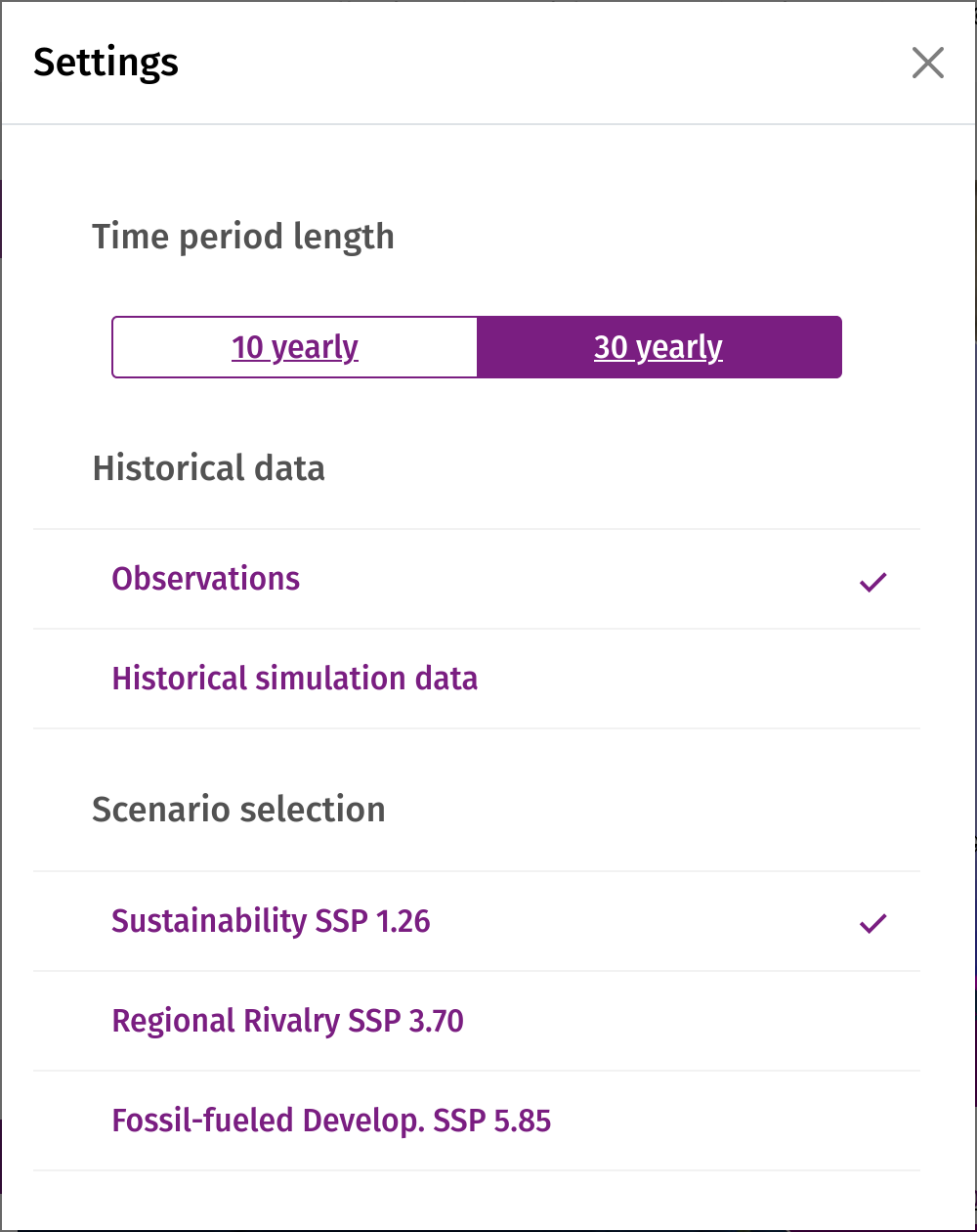
By selecting "Obsevations" in the Historical Data section of the Settings tab, you can visualise the observed data of the W5E5 dataset.
Sources:
Adler, R. F., Huffman, G. J., Chang, A., Ferraro, R., Xie, P.-P., Janowiak, J., Nelkin, E. (2003). The Version-2 Global Precipitation Climatology Project (GPCP) Monthly Precipitation Analysis (1979–Present). Journal of Hydrometeorology, 4(6), 1147–1167. doi:10.1175/1525-7541(2003)004<1147:tvgpcp>2.0.co;2
Cucchi, M., Weedon, G. P., Amici, A., Bellouin, N., Lange, S., Müller Schmied, H., Hersbach, H., & Buontempo, C. (2020). WFDE5: bias-adjusted ERA5 reanalysis data for impact studies. Earth System Science Data, 12(3), 2097–2120. https://doi.org/10.5194/essd-12-2097-2020
Hersbach, H., Bell, B., Berrisford, P., Hirahara, S., Horányi, A., Muñoz‐Sabater, J., Nicolas, J., Peubey, C., Radu, R., Schepers, D., Simmons, A., Soci, C., Abdalla, S., Abellan, X., Balsamo, G., Bechtold, P., Biavati, G., Bidlot, J., Bonavita, M., … Thépaut, J. N. (2020). The ERA5 global reanalysis. Quarterly Journal of the Royal Meteorological Society, 146(730), 1999–2049. https://doi.org/10.1002/QJ.3803
Lange, Stefan (2019): WFDE5 over land merged with ERA5 over the ocean (W5E5). V. 1.0. GFZ Data Services. https://doi.org/10.5880/pik.2019.023
Lange, S.: ISIMIP3BASD v2.4.1, https://doi.org/10.5281/zenodo.3898426, 2020.
Historical Simulation Data
To validate climate models, past climatic conditions are simulated and compared with observed data. An important indicator for validating the reliability of future climate projections from models is the simulated temporal and spatial change in global mean surface temperature from pre-industrial times to the present.
Part of the entry card to participate in the Coupled Model Intercomparison Project (Phase 6) is the historical simulation. It was added to Diagnosis, Evaluation, and Characterization of Klima (DECK) for a better seperation between CMIP and a specific phase, in this case CMIP6.
They also serve as a benchmark for CMIP6-Endorsed Model Intercomparison Projects (MIPs).
The simulations start at arbitrary equilibrium conditions from the pre-industrial control experiment (piControl). Then, various time-dependent forcings, consistent with CMIP6, such as greenhouse gas emissions, land use forcings, aerosols, solar forcing and others are fed into the models. These then generate a hindcast of historical conditions. CMIP6 historical simualtion cover the time period from 1850 to 2014.
By selecting "Historical Simulated Data" in the Historical Data section of the Settings tab, you can visualise the past simulations of the climate models.
Sources:
Eyring, V., Bony, S., Meehl, G. A., Senior, C. A., Stevens, B., Stouffer, R. J., and Taylor, K. E.: Overview of the Coupled Model Intercomparison Project Phase 6 (CMIP6) experimental design and organization, Geosci. Model Dev., 9, 1937-1958, doi:10.5194/gmd-9-1937-2016, 2016.WGCM CMIP6
Bandwidth
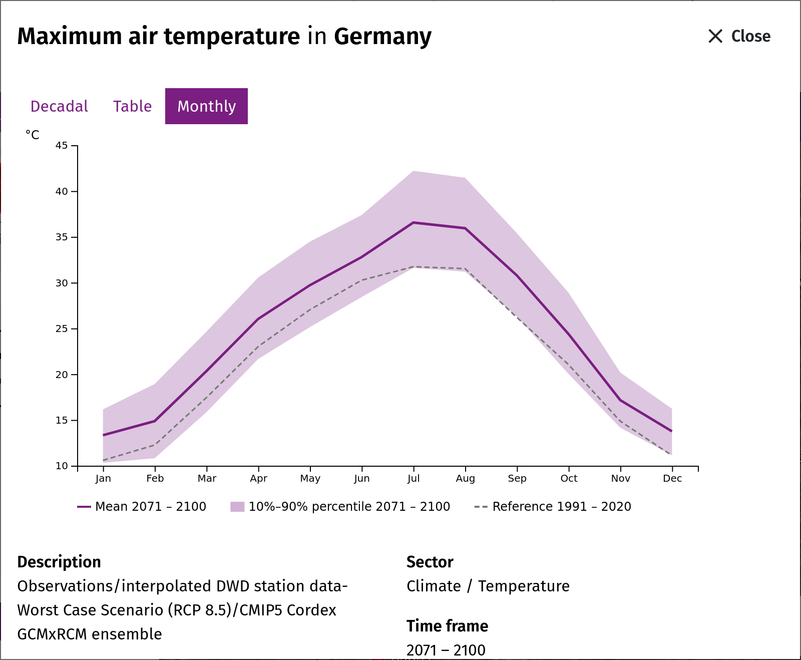
The regional climate model ensemble available from Impact3b is relatively small. That's why model uncertainty and internal (year-to-year) variability were brought together, sorted and the value at which 10%, 50% and 90% of all values are below, are described to estimate the bandwidths (50s percentile on the map, 10s, 50s and 90s percentile in the time series diagram).
For a 30-year period and a model ensemble of 4 simulations, this means a available pool of 5 x 30 = 150 annual values for the respective climate indicators.
Agricultural Parameters
The agricultural parameters are crop-specific and consist of area, production and yield data aggregated across the selected spatial scale and time period. Publicly available agricultural data in the Sahel is sparse: A tradeoff between spatial resolution and temporal range is present in many datasets, which either are spatially coarse but contain a long time series (e.g. FAOSTAT), or are spatially fine (down to the household level, e.g. RHoMIS) but are only conducted ad-hoc in single years. Additionally, data collection methodology is seldomly illuminated in the documentation of the available datasets, complicating assessments of relative accuracy and thus comparability. This is especially relevant as different datasets rarely agree with each other, often exhibiting significant differences! Another issue is the inconsistent categorisation of spatial administrative units, with some countries (e.g. Niger) having recently changed their administrative divisions or using unclear definitions based on local names and agricultural practice (e.g. Mauritania).
As a result, we have decided to aggregate data from all available sources in order to provide the most comprehensive spatial and temporal coverage possible. Depending on the spatial scale selected, the appropriate data, if available, will be displayed. If no other data is available for a region, the FAOSTAT national crop datasets are used.
Since there was no dataset for the entire Sahel region, agricultural parameters for zoom level 1 were aggregated (as a sum) from the datasets of zoom level 2 (national level).
Sources:
Carletto C., Jolliffe D., Banerjee R. (2014a): The Emperor has no Data! Agricultural Statistics in Sub-Saharan Africa [World Bank technical report]. Available at: http://mortenjerven.com/wp-content/uploads/2013/04/Panel-3-Carletto.pdf
Grassini P., van Bussel L. G. J., Van Wart J., Wolf J., Claessens L., Yang H., Boogard H., de Groot H., van Ittersum M. K., Cassman K. G. (2015): How good is good enough? Data requirements for reliable crop yield simulations and yield-gap analysis. Field Crops Research 177:49–63; http://dx.doi.org/10.1016/j.fcr.2015.03.004.
Schauberger B., Gornott C., Wechsung F. (2017): Global evaluation of a semiempirical model for yield anomalies and application to within-season yield forecasting. Global Change Biology 23(11): 1-15; DOI:10.1111/gcb.13738.
Crop statistics, land use and yields
Observed crop statistics: source and quality
The observed harvested areas, yields and production of the Sahel region come from two sources. For the countries (map level 2) we use the FAOSTAT domain Crops and livestock products of the Food and Agriculture Organization of the United Nations (FAO), annual values 1961–2024 (release of 31 December 2025). For the regions of Burkina Faso (2009–2018) and Cameroon (1998–2019) we use the national agricultural statistics of the two countries. The Sahel region (level 1) is the sum of the countries, counted only in years in which every country that reports a crop reports it.
FAOSTAT compiles the figures that national statistical offices and ministries of agriculture report to FAO in annual questionnaires; gaps are filled by FAO estimates and imputations. The quality therefore depends on the national agricultural surveys. In sub-Saharan Africa these surveys often rest on small samples, on areas estimated by the farmers instead of measured, and on irregular survey years; mixed cropping (e.g. millet with cowpea) makes the allocation of a field to one crop ambiguous (Carletto et al. 2015). Values of single years and short-term changes should therefore be read with caution, while the level and the long-term trend are more robust. Our extract contains, for each country, only its main crops, so not every crop has values in every country (e.g. no millet in Cameroon and Nigeria).
Red and white sorghum are reported only by Burkina Faso, per region and for 2009–2018. Their country values are the sum of the 13 regions; where a region reports production but no yield, its area is estimated from the yield of the other regions, provided such regions account for at most 2 % of the national production.
For each period the portal shows the median of the annual values (p50) and the range from the 10th to the 90th percentile (at least three years per period).
Land use: LUH2 and the Shared Socioeconomic Pathways
Future harvested areas are derived from the land-use data of the Inter-Sectoral Impact Model Intercomparison Project (ISIMIP3b), the same project that provides the climate and crop-model data of this portal. These data build on the Land-Use Harmonization dataset LUH2 (Hurtt et al. 2020), which provides consistent annual land-use maps from 850 to 2100 for the climate models of CMIP6. LUH2 distinguishes five functional crop types; ISIMIP splits them into 15 crop classes (e.g. maize, tropical cereals, groundnut, pulses, tropical roots and tubers) using the global harvested-area patterns of Monfreda et al. (2008), and provides them as shares of each 0.5° grid cell.
The future land use until 2100 (Volkholz and Novak 2026) was computed by two land-use models for three combinations of socioeconomic pathway and emission scenario: SSP1-2.6, SSP3-7.0 and SSP5-8.5 (Molina Bacca et al. 2025). From the Shared Socioeconomic Pathways (SSPs; O'Neill et al. 2017, Riahi et al. 2017) the models take the drivers of food and land demand: population, economic growth, diets and food waste, international trade, the growth of crop yields through technological progress, the demand for bioenergy and the protection of natural land (Popp et al. 2017). In short:
- SSP1 (sustainability): low population growth, less resource-intensive diets, high productivity growth and strong protection of natural land – little cropland expansion.
- SSP3 (regional rivalry): high population growth in today's low-income countries, slow productivity growth and restricted trade – food must largely be produced where it is consumed, hence strong cropland expansion.
- SSP5 (fossil-fuelled development): high incomes and consumption, rapid technological progress and global markets – growing demand partly met by higher yields.
The two land-use models are agro-economic models that allocate production and land so that the demand of each scenario is met:
- IMAGE (Integrated Model to Assess the Global Environment, PBL Netherlands Environmental Assessment Agency; Stehfest et al. 2014) couples an economic model of agricultural markets with a spatially explicit allocation of crops and grassland.
- MAgPIE (Model of Agricultural Production and its Impact on the Environment, Potsdam Institute for Climate Impact Research; Dietrich et al. 2019) is a partial-equilibrium model that meets food and material demand at minimum global cost, including investments in yield-increasing technology and land conversion.
Both models use biophysical data of the vegetation and crop model LPJmL – crop and pasture yields, water availability and carbon stocks. In the runs used here these data include the impacts of climate change, computed for five climate models (GFDL-ESM4, IPSL-CM6A-LR, MPI-ESM1-2-HR, MRI-ESM2-0, UKESM1-0-LL). This gives ten land-use runs per scenario (two land-use models × five climate models), harmonized with the historical LUH2 data.
Method: from land-use shares to harvested areas
For each country, each run and each year, the area of a crop class is the sum over the grid cells of its share times the area of the cell inside the country. The absolute model areas, however, differ from the statistics: for 2005–2014 they lie between 0.6 and 1.0 times the FAOSTAT area for maize, between 0.85 and 1.5 times for sorghum and millet together (in the countries that report both crops), and between 0.5 and 2.4 times for groundnut. We therefore use the land-use data only for the change and keep the observed level:
future area = observed mean area 2010–2019 × (area of the crop class in the year / area of the crop class in 2015)
- Crop classes: maize → maize; sorghum (incl. red and white), millet, fonio and other cereals → tropical cereals; groundnuts → groundnut; cowpea, dry peas and pulses → pulses; cassava and yams → tropical roots and tubers.
- The regions of Burkina Faso and Cameroon take the change of their country; the Sahel region is the sum of the countries.
- For each period, p10, p50 (median) and p90 are taken over the annual values of all ten runs.
- Cotton, sesame, cocoa and oil palm belong to mixed classes (other annual or perennial crops) and have no future values; countries and regions without observed areas have none either.
Limitations: the values describe land-use scenarios, not forecasts. The models project cropland; harvested area can be smaller (fallow) or larger (several harvests per year). All crops of one class change alike, so shifts between sorghum, millet and fonio are not represented. In line with Molina Bacca et al. (2025), the choice of the land-use model affects the results more than the choice of the climate model: under SSP3-7.0 MAgPIE projects a much stronger cropland expansion in the Sahel after 2050 than IMAGE, which widens the range from p10 to p90.
Future yields and production
Future yields are available for maize, millet and sorghum (for Burkina Faso also for red and white sorghum). They are derived from the crop models of the Global Gridded Crop Model Intercomparison (GGCMI phase 3), which were run within ISIMIP3b with the bias-adjusted climate of five climate models (GFDL-ESM4, IPSL-CM6A-LR, MPI-ESM1-2-HR, MRI-ESM2-0, UKESM1-0-LL) for the scenarios SSP1-2.6, SSP3-7.0 and SSP5-8.5 (Jägermeyr et al. 2021; Lange 2019).
- Maize: 13 crop models (ACEA, CROVER, CYGMA1p74, DSSAT-Pythia, EPIC-IIASA, ISAM, LDNDC, LPJ-GUESS, LPJmL, pDSSAT, PEPIC, PROMET, SIMPLACE-LINTUL5); for SSP3-7.0 only 8 of them.
- Millet: 3 crop models (CYGMA1p74, LPJ-GUESS, LPJmL).
- Sorghum, red and white sorghum: 4 crop models (CYGMA1p74, LPJ-GUESS, LPJmL, SIMPLACE-LINTUL5).
The model runs used keep crop areas and management at the state of 2015 and include the effect of rising CO2 concentrations on plant growth. For each country, the simulated yields of irrigated and rain-fed fields are averaged, weighted by the irrigated and rain-fed areas of the crop in the ISIMIP land-use data of 2015. In the Sahel countries only 0.3 to 5.5 % of these areas are irrigated, so the result is essentially the rain-fed yield.
From model yields to future yields. The model yields are not used directly: they are dry-matter yields under harmonised management, and they do not reproduce the year-to-year variations of the observed statistics (on the evaluation of these models see Müller et al. 2017). We tested this for 1980–2016 with model runs driven by observed weather; a statistical model fitted to the statistics (ABSOLUT, Conradt 2022) did not reproduce them either. Therefore only the relative change of each model run is used: the future yield of a country is its observed mean yield 2010–2019 (red and white sorghum: 2010–2018) multiplied by the ratio of the run's yield in a given year to the run's own mean of 2010–2019. Regions take the relative change of their country. A crop gets future values for a scenario only if at least two crop models are available; for SSP3-7.0 millet and sorghum therefore have no future values. Technical progress (new varieties, more fertiliser, more irrigation) is not included.
Production. Future production is the future harvested area times the future yield. Each land-use run is combined with each crop-model run that was driven by the same climate model. For the Sahel region, areas and production are summed over the countries; its yield is the summed production divided by the summed area.
Values shown. For each period, the map and the diagram show the median (p50) of the annual values of all runs and years of that period; the range covers the 10th to the 90th percentile (p10 to p90).
Crops without future values. Groundnuts, cowpea, fonio, yams, cotton, sesame, cocoa and oil palm are not simulated by any ISIMIP3b crop model; cassava and beans are simulated by only one each (LPJmL and LPJ-GUESS), fewer than the two models required. For these crops only observed yields and production are shown; their future harvested areas are shown where the land-use data contain a matching crop class.
Limitations. The values describe scenarios, not forecasts. The climate signal comes entirely from the crop models, and its future development cannot be checked against observations. The spread between crop models is large, in particular for millet and sorghum with only three or four models. Under SSP5-8.5, the median maize yield for 2071–2100 is 16 to 32 % below the observed mean of 2010–2019 in the countries with maize statistics; for millet and sorghum the changes are smaller, except in Niger, where the models simulate higher yields with more rainfall and the CO2 effect.
References
Carletto, C., Jolliffe, D., Banerjee, R. (2015): From tragedy to renaissance: improving agricultural data for better policies. The Journal of Development Studies 51(2), 133–148. doi:10.1080/00220388.2014.968140
Conradt, T. (2022): Choosing multiple linear regressions for weather-based crop yield prediction with ABSOLUT v1.2 applied to the districts of Germany. International Journal of Biometeorology 66, 2287–2300. doi:10.1007/s00484-022-02356-5
Dietrich, J. P. et al. (2019): MAgPIE 4 – a modular open-source framework for modeling global land systems. Geoscientific Model Development 12, 1299–1317. doi:10.5194/gmd-12-1299-2019
FAO: FAOSTAT, Crops and livestock products. Food and Agriculture Organization of the United Nations, Rome. Release of 31 December 2025, accessed 3 November 2026. www.fao.org/faostat/en/#data/QCL
Hurtt, G. C. et al. (2020): Harmonization of global land use change and management for the period 850–2100 (LUH2) for CMIP6. Geoscientific Model Development 13, 5425–5464. doi:10.5194/gmd-13-5425-2020
Jägermeyr, J. et al. (2021): Climate impacts on global agriculture emerge earlier in new generation of climate and crop models. Nature Food 2, 873–885. doi:10.1038/s43016-021-00400-y
Lange, S. (2019): Trend-preserving bias adjustment and statistical downscaling with ISIMIP3BASD (v1.0). Geoscientific Model Development 12, 3055–3070. doi:10.5194/gmd-12-3055-2019
Molina Bacca, E. J. et al. (2025): Future land-use pattern projections and their differences within the ISIMIP3b framework. Earth System Dynamics 16, 753–801. doi:10.5194/esd-16-753-2025
Monfreda, C., Ramankutty, N., Foley, J. A. (2008): Farming the planet: 2. Geographic distribution of crop areas, yields, physiological types, and net primary production in the year 2000. Global Biogeochemical Cycles 22, GB1022. doi:10.1029/2007GB002947
Müller, C. et al. (2017): Global gridded crop model evaluation: benchmarking, skills, deficiencies and implications. Geoscientific Model Development 10, 1403–1422. doi:10.5194/gmd-10-1403-2017
O'Neill, B. C. et al. (2017): The roads ahead: narratives for shared socioeconomic pathways describing world futures in the 21st century. Global Environmental Change 42, 169–180. doi:10.1016/j.gloenvcha.2015.01.004
Popp, A. et al. (2017): Land-use futures in the shared socio-economic pathways. Global Environmental Change 42, 331–345. doi:10.1016/j.gloenvcha.2016.10.002
Riahi, K. et al. (2017): The Shared Socioeconomic Pathways and their energy, land use, and greenhouse gas emissions implications: an overview. Global Environmental Change 42, 153–168. doi:10.1016/j.gloenvcha.2016.05.009
Stehfest, E., van Vuuren, D., Kram, T., Bouwman, L. (eds.) (2014): Integrated Assessment of Global Environmental Change with IMAGE 3.0. Model description and policy applications. PBL Netherlands Environmental Assessment Agency, The Hague.
Volkholz, J., Novak, L. (2026): ISIMIP3b Future Land Use Input Data (version 1.0). ISIMIP Repository. doi:10.48364/ISIMIP.848297